To a robot with emotion, navigation is a crucial aspect of its behavior because it is its only way of physical movement. The way a robot moves may be indicative of its emotional state or its feelings towards humans. However, to express such a complex behavior, the robot must be able to plan path and move freely and quickly. With only motor speeds to control and encoder values to check, there must be code built that can make and adjust a robot’s motion on the fly. This blog post will go over the implementation of trapezoidal profile in robot navigation as well as error control needed to fine-tune such implementation.

Trapezoidal Profile

Let’s say that we have a robot with only two velocities: 1 and 0. 1 is full speed and 0 is at rest.  While the robot’s behavior would be fairly predictable and uniform, whenever the robot changes velocity it would produce a jerk in motion. That is because the instantaneous change from full speed to 0 speed or vice versa would result an incredibly large magnitude in the robot’s acceleration, and Newton’s First Law of Motion would dictate that the robot would wobble from the sudden change in velocity. This problem would be further aggravated if the robot has three velocities: 1, 0, and -1. The change from maximum positive velocity to maximum negative velocity would create an acceleration spike that’s twice as large as the previous example. The robot’s motion is not be pretty and neither is your captured image. The jerk could disrupt some of the robot’s camera functions such as face detection and skeleton tracking.

In order to reduce the jerks, the robot must be able to produce a range of velocities, allowing it to speed up and slow down over time. This is the main idea of trapezoidal profile. On the graph of velocity vs time, the robot’s motion must be shaped like a trapezoid with a bottom base higher than the top base. Instead of having sudden jumps in velocities, the robot’s motion must have a section where its speed increases due to a constant positive slope/acceleration, a section where its speed is constant and acceleration is 0, and a section where its speed decreases due to a constant negative slope/acceleration. This acceleration value is defined arbitrarily, and as long as the change in time is kept constant, it can be treated as the constant change in velocity (a = delta v). However, in no circumstance can the robot’s change in velocity be higher than the defined delta v. This essential rule is the basis of trapezoidal profile no matter how many different velocities the robot intends to switch to.

In addition to reducing jerks, trapezoidal profile can also improve accuracy. As the robot is able to control its distance better at lower speed, trapezoidal profile causes robots to move slower when it is able to reach its destination, allowing it to fine-tune its motion and reduce error in its position.

Pseudocode for trapezoidal profile:

loop {
    ...
    if velocity >= velocity_limit
        velocity = velocity_limit
    else
        velocity += delta_v
}

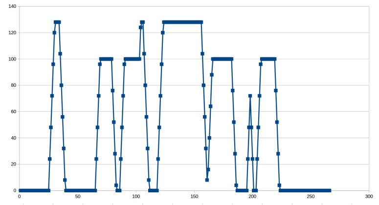
As seen from the graph of speed vs time posted, no matter what speed the robot is traveling at, its motion is fairly trapezoidal.

Feedback Loop

Although trapezoidal profile can smoothen a robot’s path, errors could still exist in the robot’s motion. These errors are the difference between the robot’s ideal position and its actual position and are mostly caused by friction. In order to make the actual position, the robot must be able to adjust its speed to reduce the amount of error. For example, if a robot actually moved farther than it intended, it should travel slower to reduce error. On the other hand, if the robot moved less than intended, it should travel faster. While our encoder values allow us to check the actual position of the robot, the motor speeds can be used to calculate our intended position. We will use a feedback loop between the encoders and the motor to control our error. The following block diagram shows our feedback loop in detail.

The difference between the intended position and the actual position is the error value. This difference will then be multiplied by a k-value known as the gain, a proportion that controls how much of the error would have effect on the motor speed. The total value would be added onto the existing motor speed and give us the actual motor speed. For example, if the intended position is the actual position, error is 0, so actual motor speed is the intended motor speed. If distance traveled is less than expected and the intended position is greater than the actual position, then a positive value would be added onto the motor speed to make the robot go faster. Otherwise if robot traveled farther than expected and the intended position is less than the actual position, a negative value would be added onto motor speed, making the robot go slower. This feedback loop ensures that the robot would travel at the speed to reduce the amount of error in its position.

Pseudocode:

loop {
    ...
    // a is positive when speeding up, negative when slowing down
    if v > vlim
        v = vlim
    else 
        v += delta_v
    if (abs(p_d - p_i) < v) 
        p_i = p_d
    else 
        p_i += v
    e = p_a - p_i
    ev = k(p_a - p_i)
    // add ev to current velocity
    ...
}

As with all the other constants used, the gain (K-value) is an arbitrary value defined by the user. If your robot travels too slowly, simply increase the gain and acceleration/delta-v value to make it react faster.